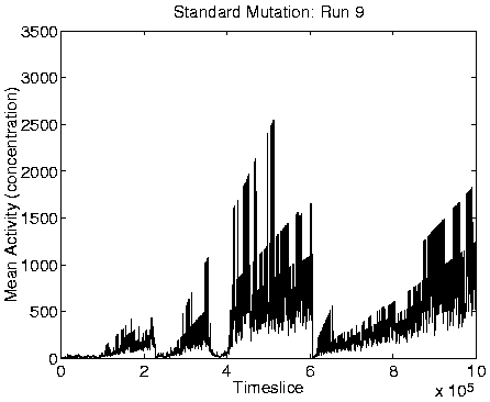
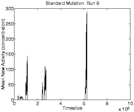
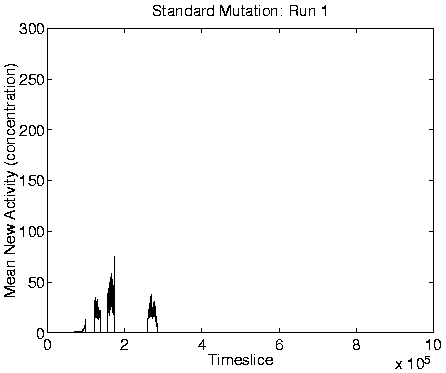
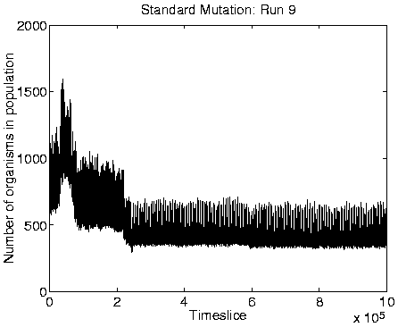
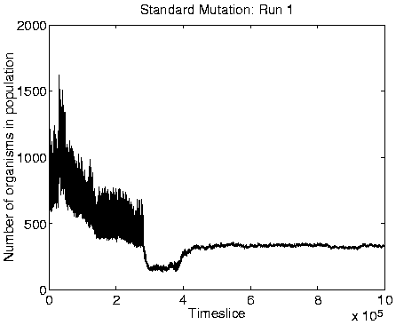
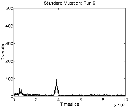
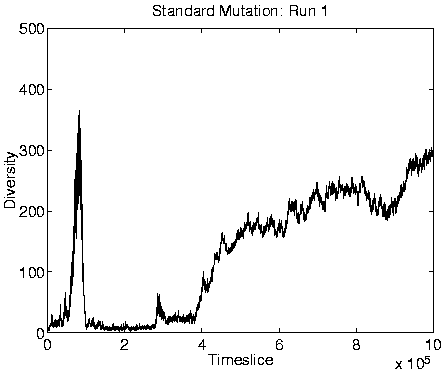
From the measures we looked at, reliable indicators of Class 1
dynamics were a combination of zero Mean Cumulative Activity
(
![]() ), zero Mean New Activity (
), zero Mean New Activity (
![]() ), stable
population size, high diversity (of the same order as the population
size), and high program length. Graphs of these measures for a typical
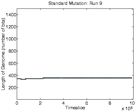
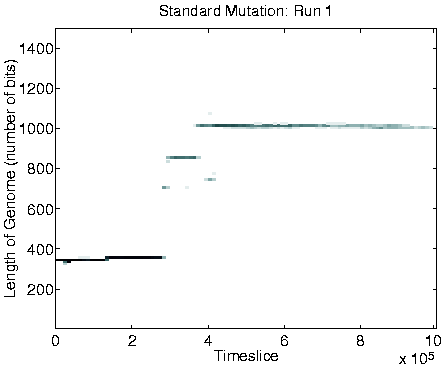
run showing Class 1 behaviour are shown in Figure 6.9,
alongside the corresponding graphs for a run showing Class 2
behaviour.
), stable
population size, high diversity (of the same order as the population
size), and high program length. Graphs of these measures for a typical
run showing Class 1 behaviour are shown in Figure 6.9,
alongside the corresponding graphs for a run showing Class 2
behaviour.
|
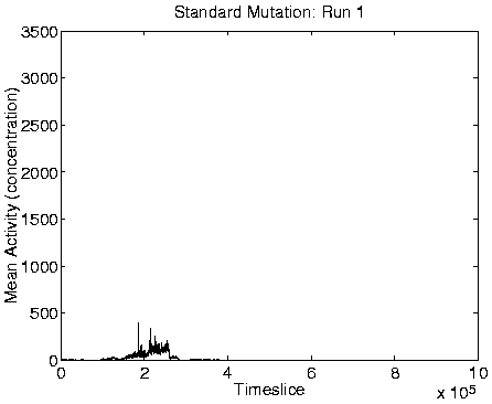
Analysis of these runs shows that in each one, at the time of the transition from Class 2 to Class 1 dynamics, a mutation appeared which caused a program not to stop copying instructions to its offspring after it had copied its final instruction, but rather to jump back and copy a section of itself a second time around. As a result, the offspring is approximately twice as long as its parent, but the first half of it is still a fully functional self-replication program. As long as the mutant retains the stop instruction at the end of the functional code, then the extra instructions do not get executed; they are the equivalent of `selfish DNA'. The Class 1 programs had also lost the ability to move around the environment.
Now, in Section 5.2.1 we looked at how the replication period of a program would be expected to vary as the program length increased under two different scenarios. In the first scenario, the length of the program's `copy loop' increased in proportion to the total program length, and in the second scenario, it remained constant (Figure 5.8). In the present situation, the second scenario is the case. Under these conditions, we found that the replication period of the program would actually remain fairly constant no matter how long the program was. The longer programs in these runs are therefore not at any disadvantage to shorter ones in this respect, which explains why they were able to survive. However, to explain why these longer programs not only survived, but actually flourished and rapidly displaced the shorter programs, we need to look for specific selective advantages they might have had over the shorter programs. A likely explanation is that, because they are executing more instructions per time slice (due to their greater length), they collect more energy from the environment (by executing more et_collect instructions) during each time slice. In these runs, programs can extract energy from neighbouring programs as they try to collect energy from the environment (the parameter energy_collection_scheme is set to shared), so a program that extracts a large amount of energy from the environment per time slice might kill off some of its neighbours by using all of their energy. Those programs which have least stored energy, i.e. probably the shorter programs which collect less per time slice, will run a greater risk of being killed in this way, hence the longer programs will tend to out-compete them.
If this explanation is correct, then we would expect not to see this Class 1 behaviour if longer programs were not able to execute more instructions per time slice than shorter programs. We will look into this in Section 6.4.
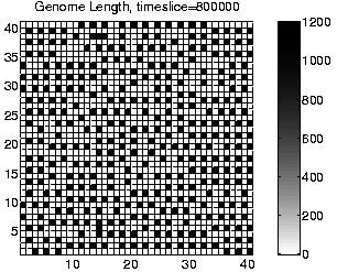
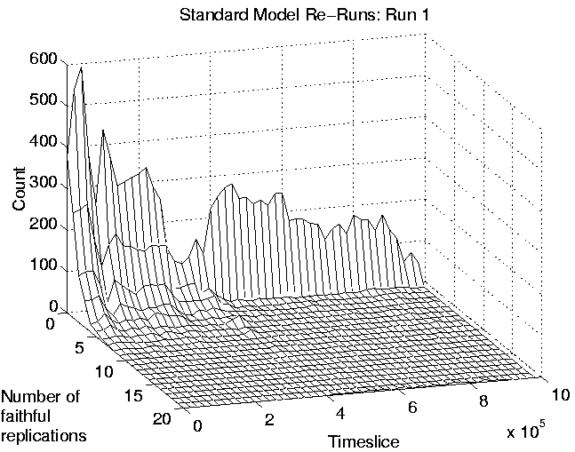
Evidence to support this explanation comes from a number of different sources. First, if the long programs are extracting energy from their immediately neighbouring programs, then we might expect the system to move towards an equilibrium position where the eight locations neighbouring each viable program are empty (because any programs which happen to find themselves in these positions will quickly be killed by energy extraction). The largest number of programs that could be stably supported in this configuration would be, for the 40 x 40 grid used in these runs, 20 x 20 = 400 (i.e. alternate positions would be occupied and empty, in both directions). Looking at the population size graphs for each of the Class 1 runs, the population size does indeed move to around 400 at the time of the transition, and stay at that level thereafter. An example plot, for Run 1, is shown in the right-hand side of Figure 6.9. More direct support for the explanation comes from the recorded `movies' of spatial distribution. A frame from the movie of program length for Run 1, at a time after the transition to Class 1 dynamics, is shown in Figure 6.10. This figure demonstrates that the spatial distribution is almost exactly as predicted (the observed pattern will never be exactly as predicted, because of the dynamic and stochastic nature of the system).
 |
A consequence of the population size being limited to 400 is that it is no longer affected by the ceiling effect discussed in Section 5.2.3. The population size therefore becomes more stable, and is not subject to the oscillations observed in the Class 2 dynamics (compare the population size graphs for Class 1 versus Class 2 dynamics in Figure 6.9).
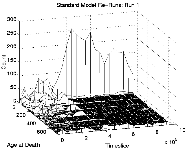
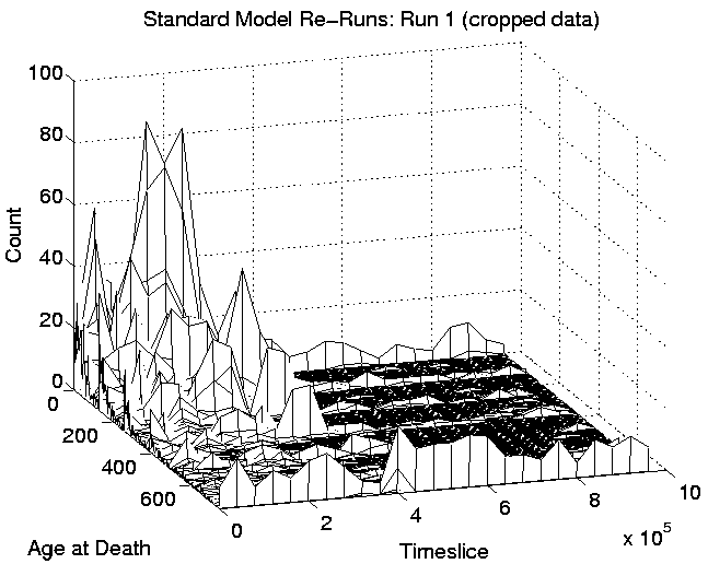
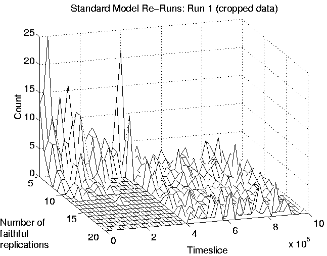
Another consequence of the spatial distribution is that the 400 or so programs which are favourably placed will tend to survive for a long time. This is because any new program that moves into a position in between two or more favourably placed programs will probably be killed off before it gets a chance to collect enough energy to fend off such attacks. The chances are weighted against the new program for two reasons: (i) being a new program, it probably has little stored energy to start with, and; (ii) because, even though at each time slice the order in which programs are given a chance to execute instructions is determined at random, there will probably be two or four favourably placed programs surrounding the new, unfavourably placed one, so it is likely that at least one of these will be executed before the new program is. Evidence for this comes from the graphs of age-at-death. These are shown, for Run 1, in Figure 6.11 (plotted in 3D for clarity). The left-hand side of this figure includes all of the recorded data, and shows that after the transition to Class 1 dynamics at around 400,000 time slices, the number of programs that are dying within their first 15 time slices increases dramatically (these are the programs placed in unfavourable positions). On the right-hand side of the figure, the same data is shown with the first row (corresponding to programs which died in their first 15 time slices) omitted, to emphasise the rest of the data (note the difference in vertical scales). This plot shows that after the transition, programs tended to live for a very short time, or a very long time, with relatively few living for intermediate durations.
|
Finally, another consequence of the transition is that those programs which are favourably placed will tend to produce more offspring (because they live longer) than did most programs before the transition. This is demonstrated, for Run 1, in Figure 6.12. Note, however, that even though these programs are producing more offspring, most of these will be killed off immediately, as already explained. The fact that few programs will produce offspring which reach the reproductive stage themselves means that lineages will not spread through the system, and explains why the diversity of the programs is very high during Class 1 dynamics. (The fact that there was presumably no selection pressure to prevent mutations in the non-functional (selfish) section of the programs must have also contributed to the high diversity.) Class 1 is therefore a degenerative state in which adaptations cannot spread throughout the population, and evolution effectively ceases.
|
 ).
).