Results

Two of the runs (numbers 2 and 8) displayed typical Class 2 dynamics for their whole duration, and four others (numbers 1, 5, 6 and 7) began as Class 2 then switched to Class 1 behaviour at some point during the run. As expected with the lower mutation and flaw rates, the timing of these transitions was generally later than in the runs reported previously, ranging from time slice 200,000 (approximately) in Run 1 to 750,000 (approximately) in Run 6.

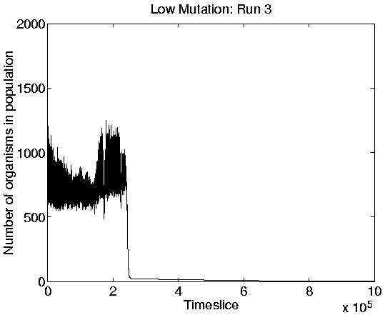
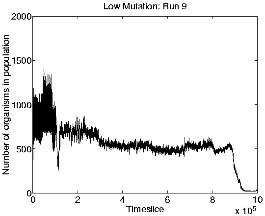
The other three runs (numbers 3, 4 and 9) displayed behaviour which had not been previously encountered. Each of these three runs initially displayed Class 2 behaviour as normal. Run 9 subsequently switched to Class 1 behaviour. However, at some later point during each run, the entire population was suddenly wiped out. (In Runs 3 and 9 a handful of programs remained, but these had lost the ability to reproduce and therefore spent the rest of the run collecting energy from the environment with no competition.) The population size graphs for runs 3 and 9 are shown in Figure 6.14.

  

Figure 6.14: Low Mutation: Population size graphs for Run 3 (left) and Run 9 (right). Both runs experience population extinctions.

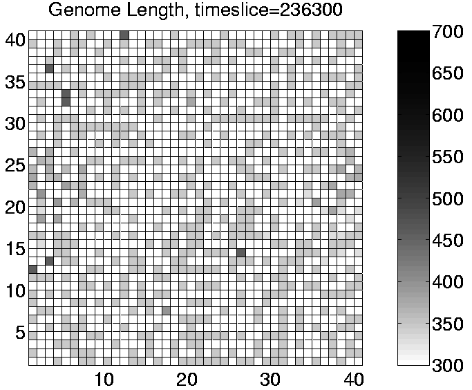
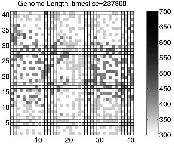
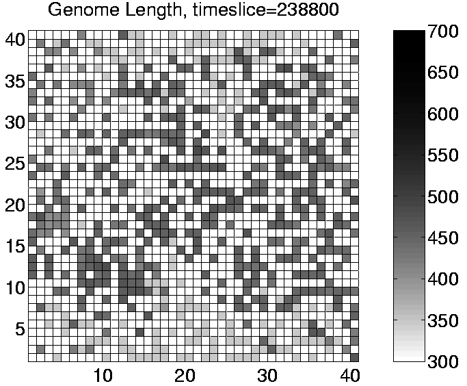
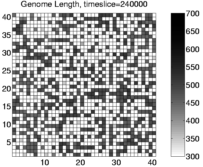
Analysis of Run 3 revealed that the population was being invaded by a sort of `cancer' mutant. The effect of this mutant was to add an extra (non-functional) instruction to the end of the program each time it reproduced. The length of the program therefore increased by one instruction (6 bits) each generation. The original mutant (342ABQQ) had actually lost an instruction (if_not_fl) from within the copy loop, which meant that it could reproduce quicker than the standard programs. This gave it an immediate benefit and enabled it to quickly spread and displace the existing programs. However, once established in the system, the mutant's offspring gradually grew longer and longer. The additional code at the end of the programs was executed, but had no significant action, and in particular, it did not include any additional et_collect instructions. The only effect of this growth was therefore to drain the program's energy store. Once the growth passed a certain size, it could completely drain the program's energy, thereby killing it. The takeover of the population by this mutant can be seen for Run 3 in the sequence of plots shown in Figure 6.15. This is a good example of the `short-sightedness' of evolution, where a variant with a short-term advantage is selected for, even though it eventually leads to the total collapse of the entire population.

  

Figure 6.15: Low Mutation: Takeover of population by `cancerous' mutant (darker squares) in Run 3. The sequence runs from top left to top right, bottom left then bottom right. The cancerous mutants can first be seen clearly as two clusters to the left and right of the central area of the top right figure. (White squares are empty.)

It is interesting that this mutant was only observed in these runs with low mutation and flaw rates. It is possible that such mutants did in fact arise in other runs, but with higher mutation and flaw rates, it is more likely that, once the detrimental effects of the mutant began to manifest themselves, a new variant would arise which corrects the defect. Such a variant would quickly displace the `cancerous' programs which have low energy reserves, and thereby save the population from extinction.