The exact procedure, which is adapted from
[Cohen 95], is shown in Figure 6.2.
The number that the procedure produces, p, is the (one-tailed)
probability of achieving a result greater than or equal to
![]() (or less than or equal to
(or less than or equal to
![]() if
if
 )
by chance under the null hypothesis. That is, p is the
probability of incorrectly rejecting the null hypothesis that systems
I and J have equal population mean scores for the measure in
question.
)
by chance under the null hypothesis. That is, p is the
probability of incorrectly rejecting the null hypothesis that systems
I and J have equal population mean scores for the measure in
question.
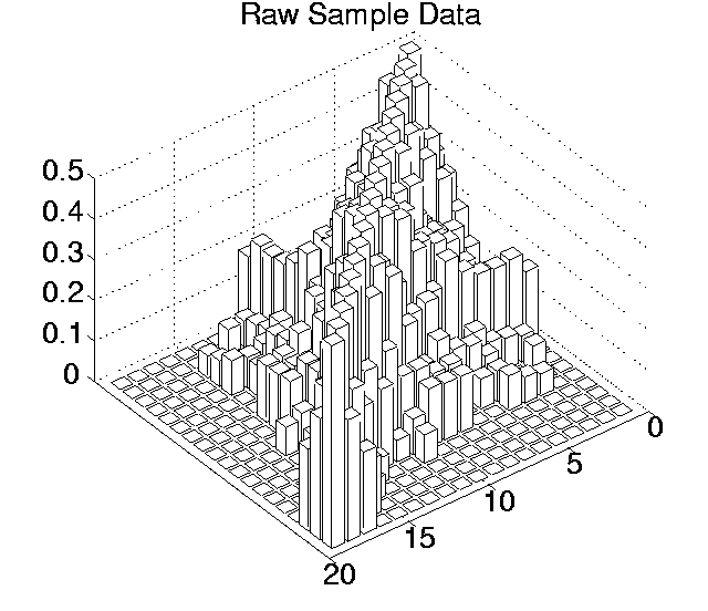
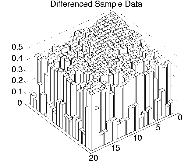
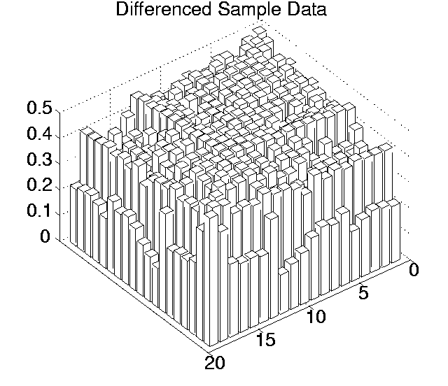
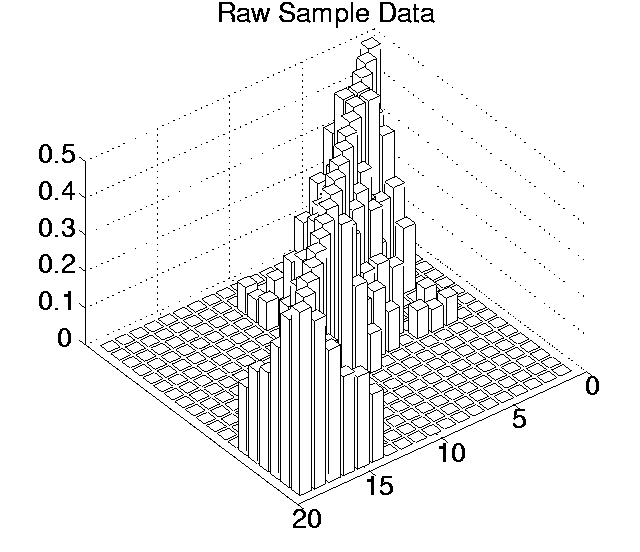
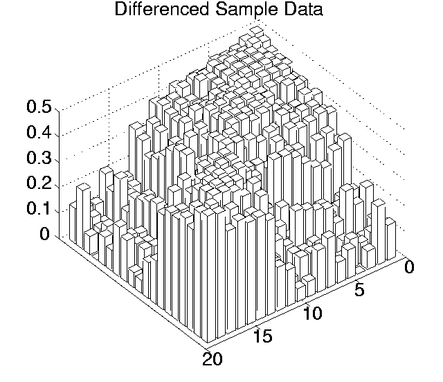
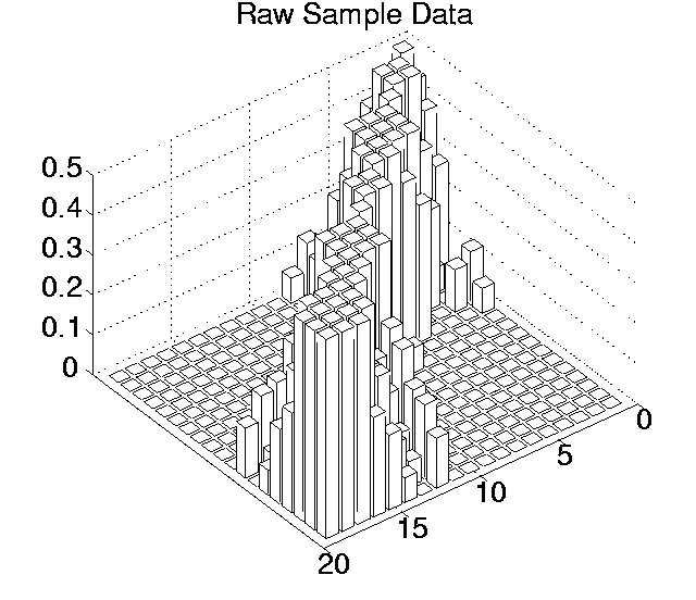
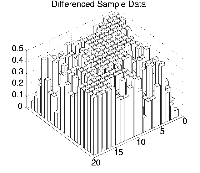
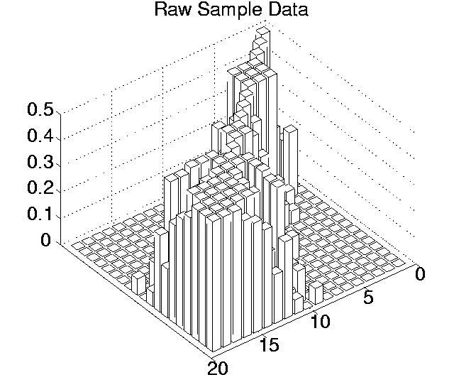
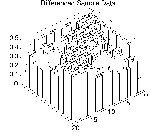
For each of the five measures being considered (Cumulative Activity, Mean Cumulative Activity, Diversity, Program Length and Replication Period), this procedure was followed for each of the 19(19 - 1)/2 = 171 pairwise comparisons between runs, for both the raw sample data and the differenced sample data.
The p values for each pairwise comparison are shown graphically in Figures 6.3-6.7. These figures show one histogram for p values obtained using raw sample data, and another for p values obtained using differenced sample data. In all of the histograms, any p value less than 0.05 is plotted as zero. Bars of non-zero height on the histograms therefore represent pairs of runs which are not significantly different from each other for the measure in question at the p=0.05 level.
(Note that, in order to emphasise the formation of various clusters of runs in these histograms, the runs in each histogram are arranged along the x and y axes in increasing order according to the mean of their 10 sample values. While this emphasises clusters in any one histogram, it means that clusters occurring in similar positions in the histograms of different measures do not necessarily represent the same runs.)
The randomisation version of the paired-sampled t test has
some advantages over other methods of investigating pairwise
comparisons (e.g. it is non-parametric), but it has the disadvantage
that it is ``virtually certain to produce some spurious pairwise
comparisons'' [Cohen 95] (p.203). Cohen suggests one way, not to
get around this problem, but at least to have some idea of the
reliability of a particular set of pairwise comparisons [Cohen 95]
(p.204). The idea is to first calculate, at the 0.05 level, how many
runs, on average, each run differed from (call this
![]() ). Then calculate a similar figure at a much more
stringent level. As we have 1024 numbers in our distribution of mean
differences, the 0.001 level is appropriate. Finally, calculate the
criterion differential,
). Then calculate a similar figure at a much more
stringent level. As we have 1024 numbers in our distribution of mean
differences, the 0.001 level is appropriate. Finally, calculate the
criterion differential,
 .
If C.D. is large, this indicates that many
significant differences at the 0.05 level did not hold up at the 0.001
level. A small C.D. value indicates that the experiment differentiates
runs unequivocally, therefore lending more weight to the validity of
the results at the 0.05 level. Table 6.2 shows
.
If C.D. is large, this indicates that many
significant differences at the 0.05 level did not hold up at the 0.001
level. A small C.D. value indicates that the experiment differentiates
runs unequivocally, therefore lending more weight to the validity of
the results at the 0.05 level. Table 6.2 shows
![]() ,
,
![]() and C.D. for each measure, and
for both raw and differenced sample data.
and C.D. for each measure, and
for both raw and differenced sample data.
Table 6.2 reveals a number of interesting results. The most striking is the difference in the results of using raw sample points compared with differenced sample points.
Using raw data, the average number of runs that any particular run was significantly different to at the 0.05 level ranged from 8.42 for Cumulative Activity to 13.26 for Diversity. However, the criterion differential for all of these measures is high (ranging from 6.21 for Mean Cumulative Activity to 12.32 for Program Length). This suggests that the validity of the figures at the 0.05 level are questionable, and the true figures are probably somewhat lower than those calculated. Having said this, the average number of runs that any particular run was significantly different to, even at the 0.001 level, was non-zero for three of the measures (Cumulative Activity, 2.11; Mean Cumulative Activity, 4.11; Diversity, 6.32).
Using differenced data, the results have a very different look. In only two measures were any runs significantly different from any others even at the 0.05 level (0.11 for Cumulative Activity and 0.42 for Diversity), and both of these vanished at the 0.001 level. In other words, these figures suggest that, for all of these measures, starting off at any point during any of the runs, the amount the measure changed over a given period was not significantly different compared to any of the other runs.
|
|
|
|
|
|
![\begin{figure}
\framebox[\textwidth][c]{\parbox{0.9\textwidth}{
\small
\begin{en...
...}\item $p = (C / 1024)$\end{enumerate}\end{enumerate}\normalsize
}}
\end{figure}](img96.gif)